Forecasting with Multiple Temporal Aggregations. Part 1: Uncertainty and Forecast Combinations

Daily Forecasting Problems.

What if I tell you that the way you are looking at a time series might be incorrect?

And yeah, I am not a lunatic.

But let’s clear some things out first. By “looking” I mean sampling a time series at a specific frequency. How are we certain that the original frequency of a time series is the best choice to fit our favorite model? Attention: by original, I refer to the frequency they provided us with. Just because we are given a time series sampled during specific intervals (days, weeks, months, etc…) does not mean that we should blindly assume that it’s the best frequency to model our data.

Hold on, hold on.

This idea introduces an additional layer of complexity into our forecasting pipeline. During every forecasting task, we are looking for the single “best model”, which will perfectly approximate our time series at hand. Then we just fit the model to a training sample, get its parameters optimized, and finally hit the forecast button. And now, I also suggest identifying the “optimal frequency” to do that. No thank you. I have enough problems in mind.

Well, I am sorry to spoil it for you, but identifying a single “best” model to approximate a data generation process is a very, very hard problem. Due to the complexity of the actual data-generating processes and the time-varying components of a time series (eg trend, seasonality, etc), it’s unlike that an observed time series is produced by a simple process that can be easily approximated through some equations. Based on that, identifying this so-called “optimal” model is a process carrying high degrees of uncertainty. Turning our focus and our recourses into a task high on uncertainty can be very costly. Yeah, money-wise costly.

Let's try to understand where does the uncertainty come from.

A Dive into the Uncertainty.

Well, I am pretty sure that everyone familiar with forecasting (and predictive analytics in general) has heard the word uncertainty before. I am also certain that a primary objective of almost every forecasting application is to quantify and mitigate this uncertainty. If not, do me a favor and revise your project’s structure. But before going into details, let’s consider:

Which exact uncertainty are we trying to mitigate?

According to the literature, there are three types of uncertainty. Namely, data uncertainty, parametric uncertainty, and model uncertainty [1]. What’s the difference between these three quantities? You might think that we are going a bit out of track here but please, stay with me. In order to understand the actual benefits of Multiple Temporal Aggregations, we first have to understand what problem they are designed to solve.

I will try to separate the three uncertainty quantities with a simple example, originally narrated in [13]. Let’s assume we want to forecast the demand for coffee in our beloved cafeteria next to our house.

To simplify the example, we assume that the demand is independent of any variable that can generally affect the need for coffee (eg past demand, time of day, price, weather, etc). So we have a constant, true demand of, say 50 coffees per day, plus/minus some randomness. We assumed that demand is independent of everything, so we only have to estimate its mean value. Any fluctuations are just a product of noise. Since we cannot predict these (otherwise I would have won the lottery), we rely on safety stocks to ensure that the daily demand is mostly satisfied. But more on that later.

In simple terms, we have the correct model: f(x) = c + ε with c∈ ℤ, but we don’t know the value for its only parameter c. Epsilon term ε stands for the randomness (noise) of the time series. To simplify the example (yes, even more) we also assume that ε is normally distributed. So far so good. By simplifying the example we have easily dealt with model selection uncertainty. But, we still have to find a solution to deal with data and parametric uncertainty.

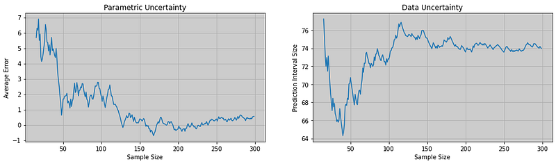
The true coffee demand is given in Figure 1. The final prediction is the mean of the observed demand. I provide three examples with different historical sample sizes. As any statistician, econometrician, data scientist, or machine learning engineer would know (feel free to add any other job title here), fitting a model to a bigger training sample results in more accurate parameter estimation. Well at least most of the time, and that’s only half the story. In turn, this (usually) results in more accurate predictions. Please, before making this a poster on any wall, watch out for uncurated and/or biased data, outdated information, and several other data issues. No doubt, parametric uncertainty is correlated to the sample size. A bigger sample size will (probably) give a better approximation of the actual value of c.

Let's get more data then!

Unfortunately, this is not the case with data uncertainty. A higher sample size does not mitigate the uncertainty originating from the model’s inability to capture the data-generating process. Either the capacity of the model is too low and/or the given data is too difficult (random) to be forecasted. In our case, since we know the correct model, coffee demand is just too difficult to be perfectly approximated. To account for how the overall uncertainty is mapped into our predictions, we use Prediction Intervals.

Definition alert!

A Prediction Interval (PI) gives a range of values that the future quantity is likely to lie in between with a specific degree of confidence [7]. PIs are very important in decision-making. For example, in inventory management, the width of the PI affects the size of the safety stock kept to satisfy a predefined service level. In money language, the higher the uncertainty, the wider the PI and in turn, the size of the safety stock. Keeping units in inventory is not cost-free. A higher safety stock increases inventory holding costs. Yeah, high uncertainty => more money in inventory.

But enough with definitions. Back to graphs. Figure 2 shows the correlation between uncertainty and sample size. Remember! We have dealt with model selection uncertainty. Clearly, an increased sample size reduces the point forecast error indicating better parameter estimation and (in our case) better point forecast. However, it does not account for the overall forecast uncertainty (mainly data uncertainty) captured by the width of the PI.

Quick Note: These are very naive evaluation methods used on a simplified example!

Now that we have distinguished the different sources of uncertainty and their importance, let’s jump into the real world where coffee demand depends on several factors. In reality, we never get the correct model nor the correct values for its parameters. Instead, we look for a model that can adequately capture all the factors that contribute to the variations of the given time series. In our cafeteria example, a candidate model can be formulated as follows:

Here, s(t) stands for seasonality, p(t) for the price, w(t) for the weather, and P(T) for promotions. Parameters c1, c2, c3, c4, and c0 are to be estimated. As before, ε represents the randomness of the time series. Equivalently, we can define any model (linear or non-linear) which includes more (or less) factors that might affect the demand for coffee. The better the model selection, the better it fits the given time series. However, it should be noted that parametric uncertainty increases as we add more factors to our model. Eventually, we look for a model that can capture the variance of the time series and be “economic” on its parameters. Or, we have a huge, high-quality training sample and unlimited computational resources. In that case, parametric uncertainty is robust to the addition of extra parameters. Well, guess what, in reality, this is rarely the case.

In real-world applications, finding a good enough forecasting model that balances the aforementioned is a major challenge. A quick note here. If you believe you have a “perfect” model that can “optimally” approximate data on any given task and return a “perfect” prediction, then you are very good at this task and you should stop reading here. Instead, go look at your magic sphere and tell me when my favorite football team will win the league. Also, if you have enough spare time and recourses to look for the “most good-enough” model on any task, then again the following should not concern you.

Otherwise, let’s keep going.

The Lazy Forecaster. How to deal with uncertainty while being lazy??

Introduction to Forecast Combinations.

Given the stated challenges and the fact that we humans tend to be lazy (well, most of us) in front of cognitive-intensive problems, we look for workarounds to avoid the model-selection problem and minimize our effort. Originating from the seminal work of Bates and Granger [2], forecast combinations have been the most promising solution in mitigating uncertainties and bypassing the problem of model selection. For a detailed review of the field, readers are referred to [3] while for theoretical details I highly recommend the work of [4] and [5].

To briefly summarize the main benefits of forecast combination: (i) Combining multiple forecasts relaxes the dependence on a single “best” forecasting model that is difficult to be estimated. (ii) The variance Var(ε_c) of the combined errors ε_c = g(ε1, ε2) is reduced given a favourable covariance. A Quick statistics lesson. Errors are distributions. When combining, we use a covariance term to measure how similar the two errors move. (iii) Multiple empirical findings point to enhanced prediction accuracy when combing multiple forecasts.

Well, this is excellent news.

Ok, but how do we get these benefits in practice? How do we actually combine these forecasts? Quick, (lame) answer: Go and scan the literature. There is a vast number of published sophisticated combination approaches with different ways of estimating the combination weights. People will think that I am joking here. If I have to look for all these well-designed combination approaches, try them out and pick the best, I could just spend my recourses on finding the “best” model. You told me that by combining forecasts I could just be lazy and save time.

The Grant Paradox.

Despite the delicate work of researchers over the past 50 years and a significant number of well-written and deeply researched papers, in practice, taking the simplest combination estimators seems like the best approach. Multiple literature findings and empirical results suggest that taking the mean (or the median) to combine uncorrelated forecasts works (surprisingly) very well. Consider the following (linear) combination formula:

where wi are the combination weights for forecasts Fi. As you probably figured out if you are paying attention, introducing additional parameters wi into the forecasting pipeline inherently adds extra parametric uncertainty. It also requires extra computational time and resources for their estimation. Extra parameters also mean extra sources of errors. Intuitively, how are we certain that the sophisticated combination approaches described in the papers are the “best” in every forecasting scenario? They might work on one application but will they work on mine?

Ahh, more questions and no answers. More uncertainty.

On the other hand, simply taking the average of multiple predictions does not introduce any sources of errors. We do not have to make any extra estimations since we are using fixed weights. Also, [4] shows that using fixed weights results in reduced variance compared to taking the “optimal combination” approach (optimal in terms of least squares). Most importantly though, empirical evidence shows that fixed weights work very well in practice. Sometimes, these simple estimators even outperform very elegant combination approaches. Using the mean (or the median) seems more than enough to combine our forecasts.

Good, now that we have identified how to combine, let’s look at a crucial pitfall. Should we be concerned about the quality of the predictions we are combining?

Yes. Inaccurate initial predictions “harm” forecast combinations. This makes sense right? In the cafeteria example, if we combine a 60 and a 40 we “hit” our demand mean of 50. But if we combine a “bad” forecast of 101 and an “excellent” of 49 we end up at a “poor” prediction of 75. Well, that’s an extreme oversimplification, but you get the idea. Another point is the diversity of the predictions. Combining two overconfident forecasts of say 65 and 70 will give another overconfident prediction of 68. On the other hand, when combining diverse forecasts, any biases or errors in individual forecasts may cancel each other out, resulting in a more accurate overall prediction. In general, combining accurate and diverse forecasts results in reduced error variance Var(ε_c) and thus, mitigating uncertainty. But this raises the million-dollar question.

How do we come up with diverse forecasts while ensuring they are not inaccurate?

With this question, I conclude Part 1. I strongly encourage you to keep this question in mind and search for possible answers. To summarize, literature contains a significant number of empirical (and theoretical) evidence pointing to the benefits of forecast combinations when properly used. In Part 2, I will try to provide answers to the questions raised in this article. We are also going to take a first look at Multiple Temporal Aggregations :).

Part 2 is available here:

References

[1] Kourentzes, N., Barrow, D. & Petropoulos, F. (2019), ‘Another look at forecast selection and combination: Evidence from forecast pooling’, International Journal of Production Economics 209, 226–235.
[2] Bates, JM and Granger, CWJ (1969). The combination of forecasts. Journal of the Operational Research Society 20(4), 451–468. DOI: 10.1057/jors.1969.103.
[3] Wang, X., Hyndman, R. J., Li, F., & Kang, Y. (2022). Forecast combinations: an over 50-year review. arXiv preprint arXiv:2205.04216.
[4] Claeskens, Gerda, et al. “The forecast combination puzzle: A simple theoretical explanation.” International Journal of Forecasting 32.3 (2016): 754–762.
[5] Atiya, Amir F. “Why does forecast combination work so well?.” International Journal of Forecasting 36.1 (2020): 197–200.
[7] Hyndman, R.J., & Athanasopoulos, G. (2018) Forecasting: principles and practice, 2nd edition, OTexts: Melbourne, Australia. OTexts.com/fpp2
[8] Nikolaos Kourentzes, Multiple Temporal Aggregation: The story so far. Part I, 27 April 2017. URL: https://kourentzes.com/forecasting/2017/04/27/multiple-temporal-aggregation-the-story-so-far-part-i/
[9] Nikolaos Kourentzes, Multiple Temporal Aggregation: The story so far. Part II: The effect of TA. 4 May 2017. URL: https://kourentzes.com/forecasting/2017/05/04/multiple-temporal-aggregation-the-story-so-far-part-ii/
[10] Nikolaos Kourentzes, Multiple Temporal Aggregation: The story so far. Part III: MAPA. 4 July 2017. URL: https://kourentzes.com/forecasting/2017/07/04/multiple-temporal-aggregation-the-story-so-far-part-iii/
[11] Nikolaos Kourentzes, Multiple Temporal Aggregation: The story so far. Part IV: Temporal Hierarchies. 22 July 2017. URL: https://kourentzes.com/forecasting/2017/07/22/multiple-temporal-aggregation-the-story-so-far-part-iv-temporal-hierarchies/
[12] Kourentzes, N., Petropoulos, F. & Trapero, J. R. (2014), ‘Improving forecasting by estimating time series structural components across multiple frequencies’, International Journal of Forecasting 30(2), 291–302.
[13] Nikolaos Kourentzes [Lancaster CMAF]. (2021, February 15). CMAF FFT: Improving organisational forecasts and decisions with hierarchical forecasting. YouTube. https://www.youtube.com/watch?v=dpASMg2jzQY