Quickstart

In ten minutes you will build a complete Stockcast workflow for one product: forecast tomorrow's demand, turn the forecast into orders, simulate eight weeks of trading, and measure the result.

The scenario. A small shop sells 250 g packs of tea, about six a day. It orders every morning, and the supplier delivers before the shop opens. Today it has 30 packs on the shelf. Sales that cannot be served are lost. How much should it order each morning, and how well does that work?

1. Sales

Stockcast reads demand as a long table: one row per SKU and period, with the columns unique_id, date (or a period number, or both), and y. Here we make twelve weeks of daily sales, about six packs a day. In your own work this is your sales history or a demand scenario.

import numpy as np
import pandas as pd

sku, today = "tea_250g", pd.Timestamp("2026-02-01")

days = pd.date_range("2026-01-05", periods=84, freq="D")
sales = pd.DataFrame({
    "unique_id": sku,
    "date": days,
    "y": np.random.default_rng(3).poisson(6, len(days)),
})
past, future = sales[sales["date"] <= today], sales[sales["date"] > today]

sales.head(3)

  unique_id       date  y
0  tea_250g 2026-01-05  4
1  tea_250g 2026-01-06  5
2  tea_250g 2026-01-07  9

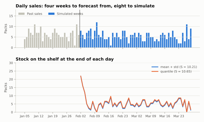
Today is 1 February. The four weeks up to today are the past we forecast from; the eight weeks after it are the future we will simulate.

2. A forecast

Every morning the shop needs a forecast of tomorrow's demand, with its uncertainty. Your forecasting model supplies it, in whichever form it produces. Here we stand in for a model with the last four weeks of sales, and state the forecast in two common forms at once:

last_4_weeks = past["y"].tail(28)
forecast = pd.DataFrame({
    "unique_id": [sku],
    "date": [today + pd.Timedelta(days=1)],   # the day it forecasts
    "fh": [1],                                # one step ahead
    "mean": [last_4_weeks.mean()],            # a moving average ...
    "std": [last_4_weeks.std()],              # ... and its spread
    "q95": [last_4_weeks.quantile(0.95)],     # or a 95% quantile forecast
})
forecast

  unique_id       date  fh      mean       std    q95
0  tea_250g 2026-02-02   1  6.357143  2.344644  10.65

• mean and std: a point forecast (the four-week moving average) and how much a day's sales vary around it.
• q95: a quantile forecast. Tomorrow's sales stay at or below 10.65 packs on 95% of days.

3. Opening stock

InventoryStateDataFrame holds everything the shop knows about its stock: what is on the shelf, what is on order, and what is owed to customers.

from stockcast.core import InventoryStateDataFrame

shelf = InventoryStateDataFrame.from_observed(pd.DataFrame({
    "unique_id": [sku],
    "date": [today],     # the day the shelf was counted
    "on_hand": [30],     # packs on the shelf
}))

4. A policy

The order-up-to policy reviews stock every period and orders enough to bring the inventory position back up to a level \(S\):

\[ q_t = \max\bigl(0,\; S - \mathit{IP}_t\bigr), \qquad \mathit{IP}_t = \text{on hand} + \text{on order} - \text{backorders}. \]

The shop wants to serve tomorrow's demand on 95% of days, so \(S\) is the 95% quantile of tomorrow's demand. Like a scikit-learn estimator, a policy is configured, then fit on a forecast:

from stockcast.policies import OrderUpToPolicy

policy = OrderUpToPolicy(
    lead_time=0,             # delivered before the shop opens
    review_period=1,         # order every morning
    freq="D",                # one period is one day
    service_level=0.95,      # cover tomorrow's demand on 95% of days
    allow_backorders=False,  # a missed sale is lost
)

policy.fit(forecast, mean_column="mean", std_column="std")
policy.get_target_levels()

  unique_id  target_level
0  tea_250g     10.213739

freq="D" says one period is one day; lead_time=0 and review_period=1 mean an order placed this morning arrives before opening and covers one day. From the mean and the spread, the policy computes the 95% quantile of a normal distribution: \(6.36 + 1.645 \times 2.34 = 10.21\) packs. Given a quantile forecast instead, it takes it as it is: policy.fit(forecast, target_column="q95") gives \(S = 10.65\).

5. Simulate

SimulationEngine plays the policy forward one day at a time. Each day it receives deliveries, lets the policy order, then serves demand. We run the policy once with each form of the forecast, refitting it in between:

from stockcast.core import SimulationEngine

engine = SimulationEngine()

# From a mean and a spread, the policy computes the quantile...
policy.fit(forecast, mean_column="mean", std_column="std")
from_mean_std = engine.run(policy=policy, demand_source=future, inventory=shelf)

# ...or it takes a quantile forecast as it is.
policy.fit(forecast, target_column="q95")
from_quantile = engine.run(policy=policy, demand_source=future, inventory=shelf)

The engine reads the run length (56 days) and the day length from the demand and the policy, and scores every day. Both runs start from the same 30 packs and meet the same demand, so any difference comes from the forecast alone.

6. Read what happened

The event table has one row per SKU and day, recording every unit that moved:

events = from_mean_std.to_event_frame()
units = ["demand", "received_units", "fulfilled_units", "order_quantity", "ending_on_hand"]
events[["date"] + units].head(7).round({column: 2 for column in units})

        date  demand  received_units  fulfilled_units  order_quantity  ending_on_hand
0 2026-02-02     8.0            0.00              8.0            0.00           22.00
1 2026-02-03     6.0            0.00              6.0            0.00           16.00
2 2026-02-04     4.0            0.00              4.0            0.00           12.00
3 2026-02-05     7.0            0.00              7.0            0.00            5.00
4 2026-02-06     8.0            5.21              8.0            5.21            2.21
5 2026-02-07     9.0            8.00              9.0            8.00            1.21
6 2026-02-08     4.0            9.00              4.0            9.00            6.21

Reading the rows:

• Feb 2 to 5. The shelf holds more than \(S = 10.21\), so the shop orders nothing and sells from stock.
• Feb 6. The morning position is 5, so it orders \(10.21 - 5 = 5.21\) packs. They arrive before opening, and the shop sells 8.
• Feb 7. The position is 2.21, so it orders 8, exactly what it sold yesterday. From now on each order replaces the previous day's sales.

The orders are fractional because the target is. OrderMultiple(1, mode="adjust") rounds them up to whole packs; see Constraints.

7. Evaluate

InventoryEvaluator turns each event table into metrics:

from stockcast.evaluation import InventoryEvaluator, avg_on_hand, fill_rate

metrics = [fill_rate, avg_on_hand]
pd.concat({
    "mean + std": InventoryEvaluator().fit(from_mean_std).evaluate(metrics),
    "quantile": InventoryEvaluator().fit(from_quantile).evaluate(metrics),
}).droplevel(1).round(2)

            fill_rate  avg_on_hand
mean + std       0.99         5.30
quantile         0.99         5.69

fit selects the scoring window (here every day) and evaluate pools all SKUs into one row. Both forecasts serve 99% of demand; the quantile forecast aims a little higher and keeps about 0.4 more packs on the shelf. The picture below shows both runs.

Summary

You can swap any box on the left and keep the rest: a forecast from a real model, a ReorderPointPolicy, a supplier with random lead times, or a shelf life.

Next steps

Here an order arrives the same morning, so it only has to last one day. With a lead time of \(L\) days and a review every \(R\) days, each order must last \(H = L + R\) days, and the forecast covers total demand over that window. Walkthrough step 3 shows how, with the same tea shop.

• Walkthrough: one idea per page, from inventory state to production.
• Guide: theory and options for each building block.
• Examples: complete notebooks, including real forecasts with smooth.