Single order (newsvendor)¶

Some decisions happen once: sandwiches for today, a Christmas collection, programmes for a concert. You buy before the season, sell during it, and whatever is left has little value. This is the newsvendor problem, and SingleOrderPolicy makes that single purchase.

The economics¶

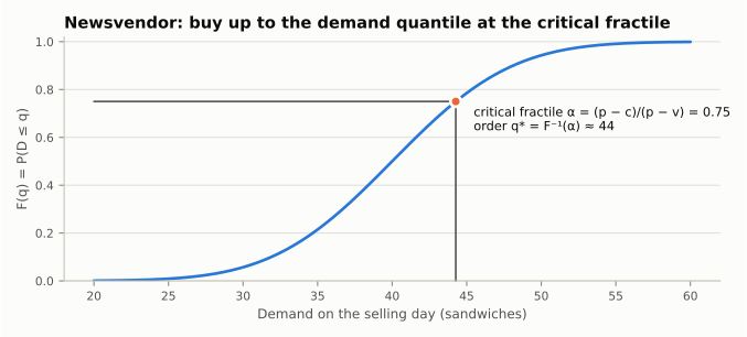
Let $p$ be the selling price, $c$ the purchase cost, and $v$ the salvage value of a leftover unit ($p > c > v$; a negative $v$ is a disposal cost). Buying one unit too few loses the margin $c_u = p - c$; buying one too many loses $c_o = c - v$. The best quantity balances the two: one more unit sells with probability $1 - F(q)$ and is left over with probability $F(q)$, so buy until $c_u \bigl(1 - F(q)\bigr) = c_o F(q)$, which gives

\[ F(q^*) = \frac{c_u}{c_u + c_o} = \frac{p - c}{p - v} = \alpha , \qquad q^* = F^{-1}(\alpha), \]

where $F$ is the forecast distribution of season demand. The ratio $\alpha$ is the critical fractile. This is the classical result for linear costs, lost sales, and a single purchase (see, for example, Silver, Pyke and Thomas, 2017).

$The newsvendor critical fractile$

newsvendor_critical_fractile computes $\alpha$:

from stockcast.policies import newsvendor_critical_fractile

alpha = newsvendor_critical_fractile(selling_price=10.0, purchase_cost=4.0, salvage_value=2.0)
alpha

0.75

Your forecast supplies $F^{-1}(\alpha)$: a quantile of demand over the whole season.

A one-day season¶

A kiosk buys sandwiches each morning, with delivery before opening ($L = 0$). History says demand is around 40 a day:

import numpy as np
import pandas as pd

from stockcast.core import InventoryStateDataFrame, SimulationEngine
from stockcast.policies import SingleOrderPolicy

history = np.random.default_rng(42).poisson(40, size=60)    # your forecast samples
quantity = float(np.quantile(history, alpha, method="inverted_cdf"))

origin = pd.Timestamp("2026-03-30")                          # last observed day
selling_day = origin + pd.Timedelta(days=1)

policy = SingleOrderPolicy(
    lead_time=0, freq="D", selling_horizon=1, service_level=alpha,
    allow_backorders=False,
    date_column="target_end",
).fit(
    pd.DataFrame({"unique_id": ["sandwich"], "target": [quantity],
                  "target_end": [selling_day]}),
    forecast_origin=origin,
    target_column="target",
)

kiosk = InventoryStateDataFrame(["sandwich"], max_lead_time=0, allow_backorders=False)
kiosk.initialize_zero(opening_date=origin)
demand = pd.DataFrame({"unique_id": ["sandwich"], "period": [0],
                       "date": [selling_day], "y": [37.0]})

result = SimulationEngine().run(
    policy=policy, demand_source=demand, inventory=kiosk,
)
day = result.to_event_frame().iloc[0]
profit = 10.0 * day.fulfilled_units - 4.0 * day.order_quantity + 2.0 * day.ending_on_hand
day[["order_quantity", "demand", "fulfilled_units", "ending_on_hand"]].to_dict(), profit

({'order_quantity': 44.0, 'demand': 37.0, 'fulfilled_units': 37.0, 'ending_on_hand': 7.0}, np.float64(208.0))

The kiosk bought 44, sold 37, and had 7 left for salvage. The profit is computed from the event table with your own prices: Stockcast records the physical flows and leaves the economics of leftovers to you.

Seasons with a lead time¶

With a lead time, the order must be placed before the season starts. The season begins when the order arrives, at demand period $\text{decision period} + L$, and lasts selling_horizon periods:

Demand period	0	1	2	3 … 7	8
With $L = 2$, a 7-period season	order placed, no demand	in transit, no demand	delivery arrives, season day 1	season days 2–6	season day 7

The target is a quantile of total season demand, and it ends at $\text{forecast origin} + (L + \text{selling horizon})\,\Delta$. The demand table contains zeros before and after the season, and the run lasts until the season ends:

L, season = 2, 7
origin = pd.Timestamp("2026-11-30")
season_totals = np.random.default_rng(1).poisson(40, size=(10_000, season)).sum(axis=1)

seasonal = SingleOrderPolicy(
    lead_time=L, freq="D", selling_horizon=season, service_level=alpha,
    allow_backorders=False,
    date_column="target_end",
).fit(
    pd.DataFrame({"unique_id": ["advent_calendar"],
                  "target": [np.quantile(season_totals, alpha)],
                  "target_end": [origin + pd.Timedelta(days=L + season)]}),
    forecast_origin=origin,
    target_column="target",
)

shop = InventoryStateDataFrame(["advent_calendar"], max_lead_time=L, allow_backorders=False)
shop.initialize_zero(opening_date=origin)
season_demand = pd.DataFrame({
    "unique_id": "advent_calendar",
    "period": range(L + season),
    "date": pd.date_range(origin + pd.Timedelta(days=1), periods=L + season, freq="D"),
    "y": [0.0] * L + [38.0, 45.0, 41.0, 39.0, 50.0, 44.0, 36.0],
})
result = SimulationEngine().run(
    policy=seasonal, demand_source=season_demand, inventory=shop,
)
events = result.to_event_frame()
events["order_quantity"].sum(), events["demand"].sum(), events["lost_sales_units"].sum()

(np.float64(291.0), np.float64(293.0), np.float64(2.0))

The shop bought 291 calendars for a season that turned out to need 293, and missed 2 sales.

Stockcast checks that the target covers exactly the season, that demand outside the season is zero, that the run observes the whole season, and that any opening pipeline arrives by the season's start.

Notes¶

The critical fractile assumes linear costs, lost sales, and no second purchase. With extra costs (disposal fees, goodwill), capacity limits, or expiry during the season, compute your own target and pass it in; the policy, engine, and event table work the same way.
A one-row weekly demand table is a one-period season; seven daily rows are a seven-period season, and the target is then a quantile of the seven-day total.

See also: Notebook 04b: daily newsvendor