Work with any timing convention¶

Papers and simulation libraries describe the same order in different words. One says "order at the end of the day, lead time 3". Another says "decide at the start of the day, lead time 2". Very often these are the same order, arriving on the same morning. This page shows how to read any description and set Stockcast so the order means what the source means. The quick reference below summarises the result; the rest of the page explains it.

Quick reference¶

You read…	Set in Stockcast
"order at the start of the period", "review, then demand"	`lead_time = L`, same decision periods
"order at the end of the period", "received at the start of t + L"	`lead_time = L - 1`, decisions one period later
"L includes one period of ordering delay"	`lead_time = L - 1`, decisions one period later
"arrives at the start of period t + l + 1"	`lead_time = l`, decisions one period later
"lead time demand over t+1 … t+L", "review time included in L"	window \(H = L\); `lead_time + review_period = L`
"the order arrives immediately after it is placed"	`lead_time = 0`

Stockcast's convention¶

Stockcast runs every period in the same order: receive, decide, then meet demand. An order placed in period \(t\) with lead time \(L\) is on the shelf before demand in period \(t + L\).

Timing of one decision

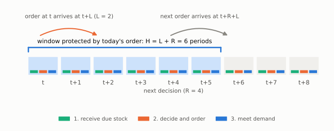
Timing: receive, decide, demand explains this clock in full. Here we only need its two consequences: a decision never sees the demand of its own period, and lead_time counts the periods from the decision to the first period the goods can sell.

The rule¶

Every convention you will meet answers two questions its own way: where the decision sits in the period, and what the lead time counts. One rule translates all of them:

lead_time = the first period the goods can serve demand − the period Stockcast decides in.

A decision "at the end of period \(t\)" is Stockcast's decision at the start of period \(t + 1\).

The second line is not an approximation. At the end of period \(t\) and at the start of period \(t + 1\) the decision has seen the same demand, up to period \(t\). In between, the only thing that happens is the arrival of goods already on order, and arrivals move stock from the pipeline to the shelf without changing the inventory position. Same information, same position, same order: when a policy uses only that position and the same fitted levels, it proposes the same quantity. Rules that also read on-hand stock or pipeline need the state check below.

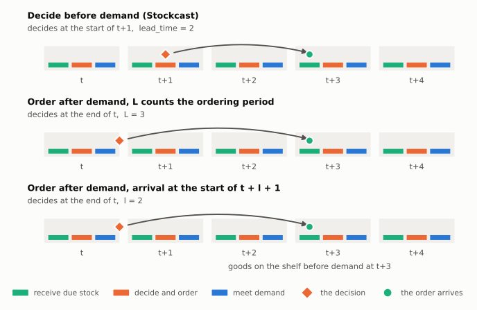
The same order in three conventions

The figure shows one order, described three ways. All three put the goods on the shelf before demand on day \(t+3\), so all three become lead_time = 2 in Stockcast.

Three questions for any description¶

Read the source with three questions in mind:

What has the decision seen? The last period whose demand it knows is its forecast origin. Stockcast decides in the period after it.
From which period can the goods be sold? Subtract the decision period: that is lead_time.
Which periods must the order cover? Until the next order can arrive: \(H = (u - t) + L\), with \(u\) the next decision. For review every \(R\) periods, \(H = L + R\). Stockcast checks your target against this window.

The rest of this page applies these questions to the conventions you are most likely to meet.

Case 1: decide at the start of the period, before demand¶

This is Stockcast's own convention, and the classic one in inventory theory. Receive what is due, review, order, then face the period's demand.

Zhu (2022, Section 3): "A possibly outstanding order arrives at the beginning of each period. The inventory position is then reviewed and an order is placed if necessary."
Janakiraman and Roundy (2004, Section 3) place the order, receive shipments, then observe and satisfy demand.
Gijsbrechts et al. (2022, Section 3): "At the beginning of any period t, the order quantity … must be decided knowing the last observed inventory on hand", and orders placed \(l\) periods earlier "are available at the beginning of period t".
van Jaarsveld and Arts (Section 3): an order placed in period \(t\) arrives "at the start of period t + τ".
Michna and Nielsen place the order "at the beginning of a period t", using demand up to \(t - 1\).

The reinforcement-learning environments for inventory control listed in the references follow it too: the agent orders, deliveries arrive, then demand is realised.

In Stockcast: use the numbers as written, lead_time = L, and decide in the same periods.

Case 2: order at the end of the period, and the lead time counts that period¶

Here demand comes first and the order is placed afterwards, at the end of the period. The lead time counts from the order to the period the goods arrive, so it includes the step from the end of one period to the start of the next.

Dejonckheere et al. (2003, Section 3): "an order placed at the end of period t is received at the start of period t+L", where "the lead-time L, consists of one time period ordering delay and \(T_p\) time periods of physical production or distribution delay".
Petropoulos, Wang and Disney (2019, Section 3.3): "the term L includes the transportation lead-time and a one sequence of events delay"; the stock balance is \(i_t = i_{t-1} + o_{t-L} - d_t\).
Michna, Disney and Nielsen (2020): "At the end of the period, the inventory level, demand and lead times of received orders are observed and a new replenishment order … is placed."
Theodorou, Spiliotis and Assimakopoulos (2025, Section 3): demand is subtracted, then an order is placed; the net stock follows \(NI_t = NI_{t-1} + Q_{t-L} - D_t\).
Chin, Cheng and Gunawan (2026, Section III-D): "Receipts precede demand; orders placed after demand arrive L months later."

Some simulation libraries use this order of events as well, and one of them notes in its documentation that a lead time one period longer matches the decide-first convention.

In Stockcast: the order placed at the end of period \(t\) is on the shelf before demand in period \(t + L\). Stockcast decides at the start of \(t + 1\), so

\[ \texttt{lead\_time} = L - 1 , \]

and every decision moves one period later: a schedule that starts at period \(0\) in the source starts at period \(1\) in Stockcast. With \(L = 1\) the goods arrive the next morning, which is lead_time = 0.

Check it on a run¶

Below, the source's rule is written as a few lines of plain Python: receive, serve demand, then order up to \(S\) at the end of the day. Next to it, Stockcast runs the same rule with lead_time = L - 1 and decisions starting one day later.

import numpy as np
import pandas as pd

from stockcast.core import InventoryStateDataFrame, PeriodicSchedule, SimulationEngine
from stockcast.policies import OrderUpToPolicy

L, S = 3, 24.0                          # as the source writes them
demand = np.random.default_rng(7).poisson(5, 12).astype(float)


def order_after_demand(demand, L, S, on_hand):
    """Receive Q[t-L], serve demand (lost sales), then order up to S."""
    pipeline, orders, stock = {}, [], []
    for t, d in enumerate(demand):
        on_hand += pipeline.pop(t, 0.0)
        on_hand -= min(on_hand, d)
        order = max(0.0, S - on_hand - sum(pipeline.values()))
        pipeline[t + L] = order
        orders.append(order)
        stock.append(on_hand)
    return np.array(orders), np.array(stock)


source_orders, source_stock = order_after_demand(demand, L, S, on_hand=15.0)

sku, opening = "flour_1kg", pd.Timestamp("2026-03-01")
policy = OrderUpToPolicy(
    lead_time=L - 1,
    schedule=PeriodicSchedule(every=1, start=1),
    freq="D", allow_backorders=False,
).fit(
    pd.DataFrame({"unique_id": [sku], "target": [S],
                  "date": [opening + pd.Timedelta(days=L)]}),
    target_column="target",
)
events = SimulationEngine().run(
    policy=policy,
    demand_source=pd.DataFrame({
        "unique_id": sku,
        "date": pd.date_range(opening + pd.Timedelta(days=1), periods=12, freq="D"),
        "y": demand,
    }),
    inventory=InventoryStateDataFrame.from_observed(
        pd.DataFrame({"unique_id": [sku], "date": [opening], "on_hand": [15.0]}),
        allow_backorders=False,
    ),
).to_event_frame()

print(pd.DataFrame({
    "demand": demand,
    "source order (end of day)": source_orders,
    "Stockcast order (next day)": events["order_quantity"].to_numpy(),
    "stock (both)": events["ending_on_hand"].to_numpy(),
}).head(7).to_string())

   demand  source order (end of day)  Stockcast order (next day)  stock (both)
0     6.0                       15.0                         0.0           9.0
1     5.0                        5.0                        15.0           4.0
2     8.0                        4.0                         5.0           0.0
3     2.0                        2.0                         4.0          13.0
4     7.0                        7.0                         2.0          11.0
5     4.0                        4.0                         7.0          11.0
6     7.0                        7.0                         4.0           6.0

Each order appears one row later in Stockcast, because Stockcast records it on the morning it is placed. The stock is the same every day. The order placed on the evening of day 0 is on the shelf before demand on day 3, which is why the stock jumps to 13 there. Both checks hold for the whole run:

assert np.array_equal(events["order_quantity"].to_numpy()[1:], source_orders[:-1])
assert np.array_equal(events["ending_on_hand"].to_numpy(), source_stock)

The target here is a fixed level, so the policy leaves service_level unset. With a forecast target you would fit it exactly as in Refresh targets as forecasts roll, with each target's origin on the last day the decision has seen.

Case 3: order at the end of the period, and the lead time is only the delay¶

Some descriptions keep the end-of-period order but count only the physical delay: an order placed at the end of period \(t\) with lead time \(l\) arrives at the start of period \(t + l + 1\). Dejonckheere et al. (2003) use exactly this quantity inside their \(L\): it is their physical delay \(T_p\), so the two counts sit side by side in one paper. Some simulation libraries describe their timing this way too.

In Stockcast: lead_time = l, with every decision one period later.

Case 4: the "lead time" already includes the review period¶

Many forecasting studies describe the order by the demand it must cover and call that span the lead time.

Kourentzes, Trapero and Barrow (2020, Section 4.2): the target sums forecasts over \(t+1, \dots, t+L\), and "L is constant and known, and any review time is included in it."
Prak, Teunter and Syntetos (2017, Section 3): the forecast is made "at the end of time N", and the lead time demand runs over \(N+1, \dots, N+L\).

That number is the window \(H\), not the delay. Choose lead_time and the review period so that they add up to it: with a review every period, lead_time = L - 1 and review_period = 1. The forecast origin is the last period the forecast has seen, as the source states.

These studies are also a good reminder of why Stockcast asks for a target over the whole window: forecast errors are correlated across the periods of a lead time, so the variance of the total is not the per-period variance times \(L\) (Prak, Teunter and Syntetos, 2017).

Case 5: zero lead time¶

When the goods are on the shelf before the demand they are meant for, the lead time is zero. Stockcast receives such an order right after the decision, before the period's customers arrive.

Dubois, Allaert and Witlox (2013, Section 2): "the lead time is zero, i.e. the order arrives immediately after the order is placed".
Gijsbrechts et al. (2022, Section 3), with \(l = 0\): the order "is immediately received and added to the on-hand inventory".
Wang, Kang, Spiliotis and Petropoulos (2026, Section 4): "Replenishment decisions are finalized prior to the start of period t+1", and the order-up-to level is a quantile of that period's forecast.

In Stockcast: lead_time = 0.

One of the simulation libraries in the references also allows an order placed after seeing a period's demand to serve that same demand. That order knows its own demand before it is placed, so it has no counterpart in a clock where decisions come before demand. Stockcast keeps that boundary on purpose.

Setting the window¶

Once lead_time is set, the window follows from the same three questions, now in Stockcast's periods:

The source	`lead_time`	Window \(H\), review every \(R\)
Case 1: decide before demand, lead time \(L\)	\(L\)	\(L + R\)
Case 2: end of period, arrival at \(t + L\)	\(L - 1\)	\(L - 1 + R\)
Case 3: end of period, arrival at \(t + l + 1\)	\(l\)	\(l + R\)
Case 4: "lead time" \(L\) includes review	\(L - R\)	\(L\)
Case 5: zero lead time, before demand	\(0\)	\(R\)

Read the window from the arrival and the next decision rather than from its name. When a description quotes a window that differs from the one its arrival and review imply, compute the level the way the source does, fit it for the window the decision actually protects, and leave service_level unset: a level computed over another span is not that window's quantile, so it should not carry that window's probability. For irregular schedules the window of each decision is \((u - t) + L\); see Decision schedules.

If a description says the stock balance is \(NI_t = NI_{t-1} + Q_{t-L} - D_t\) but the model has lost sales, check one more detail: whether \(Q_{t-L}\) arrives before or after the demand of period \(t\). Before is Case 2. After means the goods first sell in period \(t + 1\), one period later, so lead_time = L.

Backtests with dated origins¶

In a backtest each target usually carries its forecast origin: the last period its forecast saw. Keep that origin as it is. A source's order "at the end of period \(t\)" and Stockcast's decision at the start of \(t + 1\) have seen the same demand, so the target made at origin \(t\) belongs to that decision whatever the source calls the moment of ordering. Only lead_time and the window change, as in the cases above. rolling_schedule places each origin on its decision.

What the translation changes¶

When the policy, constraints and other components make the same decisions, the translation preserves the physical story: the same orders, arrivals and stock. Four details matter when comparing the records and costs.

The event table row. An order placed at the end of period \(t\) appears on Stockcast's row \(t + 1\), the morning it is placed. Order counts in a warm-up or scoring window can shift by one at the window's edge.
The edges of the run. A source's order at the end of the last period happens after the run and never reaches the shelf within it. The first decision starts one period later, as in the example.
Events at the start of a period. Stockcast's decision at \(t + 1\) comes after that morning's expiry (ShelfLife) and supplier outcomes (unreliable deliveries). A decision at the end of period \(t\) would not see them yet. This only matters when you use those features.
Rules that read the stock on the shelf. That morning's arrivals are already received when Stockcast decides. A custom policy that orders on on-hand stock alone, rather than on the inventory position, sees that morning view. So does ShelfSpaceLimit while backorders are waiting: the morning's receipt fills them, which frees shelf space without changing the inventory position.

Every run's manifest records Stockcast's own convention under run_settings["timing_convention"], so a saved result always says which clock produced it.

References¶

Chin, J. E., Cheng, S.-F., and Gunawan, A. (2026). Accuracy is not service: A decision-aware benchmark for intermittent-demand forecasting. arXiv:2609.13840
Dejonckheere, J., Disney, S. M., Lambrecht, M. R., and Towill, D. R. (2003). Measuring and avoiding the bullwhip effect: A control theoretic approach. European Journal of Operational Research, 147(3), 567–590. doi:10.1016/S0377-2217(02)00369-7
Dubois, T., Allaert, G., and Witlox, F. (2013). Determining the fill rate for a periodic review inventory policy with capacitated replenishments, lost sales and zero lead time. Operations Research Letters, 41(6), 726–729. doi:10.1016/j.orl.2013.10.006
Gijsbrechts, J., Boute, R. N., Van Mieghem, J. A., and Zhang, D. J. (2022). Can deep reinforcement learning improve inventory management? Performance on lost sales, dual-sourcing, and multi-echelon problems. Manufacturing & Service Operations Management, 24(3), 1349–1368. doi:10.1287/msom.2021.1064
Janakiraman, G., and Roundy, R. O. (2004). Lost-sales problems with stochastic lead times: Convexity results for base-stock policies. Operations Research, 52(5), 795–803. doi:10.1287/opre.1040.0130
Kourentzes, N., Trapero, J. R., and Barrow, D. K. (2020). Optimising forecasting models for inventory planning. International Journal of Production Economics, 225, 107597. doi:10.1016/j.ijpe.2019.107597
Michna, Z., Disney, S. M., and Nielsen, P. (2020). The impact of stochastic lead times on the bullwhip effect under correlated demand and moving average forecasts. Omega, 93, 102033. doi:10.1016/j.omega.2019.02.002
Michna, Z., and Nielsen, P. The impact of lead time forecasting on the bullwhip effect. arXiv:1309.7374
Petropoulos, F., Wang, X., and Disney, S. M. (2019). The inventory performance of forecasting methods: Evidence from the M3 competition data. International Journal of Forecasting, 35(1), 251–265. doi:10.1016/j.ijforecast.2018.01.004
Prak, D., Teunter, R., and Syntetos, A. (2017). On the calculation of safety stocks when demand is forecasted. European Journal of Operational Research, 256(2), 454–461. doi:10.1016/j.ejor.2016.06.035
Theodorou, E., Spiliotis, E., and Assimakopoulos, V. (2025). Forecast accuracy and inventory performance: Insights on their relationship from the M5 competition data. European Journal of Operational Research, 322(2), 414–426. doi:10.1016/j.ejor.2024.12.033
van Jaarsveld, W., and Arts, J. Projected inventory level policies for lost sales inventory systems: Asymptotic optimality in two regimes. arXiv:2101.07519
Wang, S., Kang, Y., Spiliotis, E., and Petropoulos, F. (2026). Multi-objective probabilistic forecast combination for inventory demand. arXiv:2606.04900
Zhu, H. (2022). A simple heuristic policy for stochastic inventory systems with both minimum and maximum order quantity requirements. Annals of Operations Research, 309, 347–363. doi:10.1007/s10479-021-04441-1

Simulation software whose documented conventions appear on this page: