Step 3 of 9

Forecast targets¶

A forecast says what demand might be. A policy needs something more specific: how much stock to aim for. This page shows how one becomes the other.

The protection horizon¶

The tea shop orders every \(R = 4\) days, and deliveries take \(L = 2\) days. Today's order is the last one that can arrive before the order placed at the next review. That next order only arrives \(R + L\) days from now. So today's decision has to protect demand for

\[ H = L + R = 2 + 4 = 6 \text{ days.} \]

This window \(H\) is the protection horizon. The timing page derives it day by day.

A quantile of total demand¶

Let \(D_{t}, D_{t+1}, \dots, D_{t+H-1}\) be demand over the window. The order-up-to level \(S\) is a high quantile of their sum:

\[ S \;=\; Q_{\alpha}\!\left(\,\sum_{h=0}^{H-1} D_{t+h}\right), \]

where \(\alpha\) is the target probability, for example \(0.95\). If the forecast is right, the six-day total stays at or below \(S\) with probability at least \(\alpha\). For continuous demand this is exactly \(\alpha\); for whole-unit demand the probability can be higher because quantiles move in steps.

Quantile of the sum¶

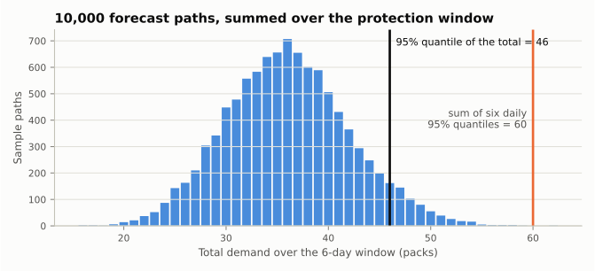
Your forecasting model can often give you a daily 95% quantile. Adding six of those does not give the 95% quantile of the six-day total. A day with unusually high sales is often balanced by a quieter day, so totals vary less than "every day at its 95% high" suggests. The picture shows it with 10,000 forecast paths:

Quantile of the sum versus sum of quantiles

import numpy as np
import pandas as pd

rng = np.random.default_rng(42)
paths = rng.poisson(6.0, size=(10_000, 6))   # 10,000 possible futures, 6 days each

quantile_of_sum = np.quantile(paths.sum(axis=1), 0.95)
sum_of_quantiles = np.quantile(paths, 0.95, axis=0).sum()
quantile_of_sum, sum_of_quantiles

(np.float64(46.0), np.float64(60.0))

Both numbers come from the same forecast, but they answer different questions. The first is what "95% protection over six days" means: 46 packs. The second would hold 14 extra packs on the shelf all the time. That is why Stockcast asks for the target of the whole window. Forecast targets has the full argument.

Computing the target¶

Every forecasting library can produce one of these. Pick the one that matches your model's output.

1. Sample paths2. A cumulative forecast3. Daily mean and standard deviation

Many models can simulate future paths: bootstrapped residuals, Monte Carlo from a state-space model, or samples from a probabilistic neural network. Sum each path over the window, then take the quantile across paths. This also captures dependence between days.

horizon = 6
target_value = np.quantile(paths[:, :horizon].sum(axis=1), 0.95)

Some models forecast the total directly. In smooth, for example, ask for the upper bound of the cumulative forecast:

from smooth import ES

model = ES(model="ANN")
model.fit(history["y"])
total = model.predict(h=6, interval="prediction", level=0.95,
                      side="upper", cumulative=True)
target_value = float(total.upper.iloc[-1, 0])

If your model gives each day's mean \(\mu_h\) and standard deviation \(\sigma_h\), and you are happy to treat days as independent and normal, Stockcast can combine them for you:

\[ S = \sum_{h=1}^{H} \mu_h \;+\; z_{\alpha}\sqrt{\sum_{h=1}^{H} \sigma_h^{2}}, \]

where \(z_{\alpha}\) is the standard normal quantile (\(z_{0.95} \approx 1.645\)). See the example below.

Target tables¶

A target is only meaningful together with the window it covers. A target table carries one row per SKU with the value and the last date it covers:

sku = "tea_250g"
opening_date = pd.Timestamp("2026-01-05")

target = pd.DataFrame({
    "unique_id": [sku],
    "target": [quantile_of_sum],
    "date": [opening_date + pd.Timedelta(days=horizon)],   # the last day it covers
})
target

  unique_id  target       date
0  tea_250g    46.0 2026-01-11

When a policy is fitted (next step), the rest follows from the policy and the date: the period length (freq), the probability (service_level), and the horizon \(H = L + R\). The forecast was made \(H\) periods before the date, on the opening date here; you can also pass it as forecast_origin, and Stockcast checks that the two agree. A target built for a different window is rejected at fit or before the run starts.

From means and standard deviations¶

Route 3 uses a forecast table with one row per future period, numbered by fh (forecast horizon \(1 \dots H\)):

from stockcast.policies import OrderUpToPolicy

daily = pd.DataFrame({
    "unique_id": sku,
    "fh": range(1, 7),
    "date": pd.date_range(opening_date + pd.Timedelta(days=1), periods=6, freq="D"),
    "mean": 6.0,
    "std": np.sqrt(6.0),
})

policy = OrderUpToPolicy(lead_time=2, review_period=4, freq="D", service_level=0.95,
                         allow_backorders=False).fit(
    daily, mean_column="mean", std_column="std",
)
policy.get_target_levels()

  unique_id  target_level
0  tea_250g     45.869122

With a mean and variance of 6 per day, the normal approximation gives \(36 + 1.645 \times \sqrt{36} = 45.9\): very close to the 46 from the sample paths.

Summary¶

A policy's target covers the whole protection window \(H = L + R\).
The target is a quantile of total demand over that window: sum first, then take the quantile.
Any forecasting model works: use sample paths, a cumulative forecast, or means and standard deviations.

Next: Policies