The simulation engine¶

SimulationEngine runs the clock. It validates every input, plays the system forward one period at a time, applies every change to stock, and returns a SimulationResult with the complete record of what happened.

`run`¶

result = SimulationEngine(verbose=0).run(
    policy, demand_source, inventory, n_periods=None,
    *, freq=None, warmup_periods=0, scoring_periods=None,
    settlement_periods=0, order_during_settlement=None,
    demand_source_name=None, random_seed=None,
    policy_schedule=None, order_constraints=None, callbacks=None,
    supply=None, processes=None,
    allow_target_reuse=True, missing_targets="raise",
)

Argument	Meaning
`policy`	A fitted policy.
`demand_source`	A demand table, or a function `period -> DataFrame`.
`inventory`	The opening `InventoryStateDataFrame`.
`n_periods`	Number of demand periods to simulate. Read from a demand table; needed for a demand function.
`freq`	Length of one period, a pandas frequency such as `"D"`. Read from the policy's `freq`; needed for a policy that has none. If given, it must match the policy's.
`warmup_periods`, `scoring_periods`, `settlement_periods`	Consecutive windows that add up to `n_periods`. Warm-up and settlement default to 0; scoring defaults to the rest and must be at least 1.
`order_during_settlement`	Whether the policy may still order in the settlement window. Needed when `settlement_periods > 0`.
`demand_source_name`	Optional label for the demand, stored in the manifest.
`random_seed`	Optional seed behind the demand, stored in the manifest.
`policy_schedule`	`{decision_period: fitted_policy}`: fresh targets at later decisions, prepared before the run. To refit a forecast during the run, see Refresh targets as forecasts roll.
`order_constraints`	A list of ordering constraints, applied in order.
`callbacks`	A list of callbacks, applied in order.
`supply`	A `SupplyModel`: suppliers, lead times, split deliveries.
`processes`	A list of inventory processes, such as `ShelfLife`.
`allow_target_reuse`	`True` (default): a policy keeps deciding until `policy_schedule` replaces it, so one target can serve many decisions. `False`: every decision needs a target fitted for it (details).
`missing_targets`	`"raise"` (default): every SKU needs a target at every decision. `"no_order"`: a SKU without a target at a decision gets no order there, flagged in `target_missing_flag`; a callback or constraint that gives it an order stops the run (details).

Only the policy, the demand, and the opening state are required. The run length and the period length come from them, and every period is scored unless you set windows. The last block switches on extra building blocks; leave them out and the run uses none of that code.

SimulationEngine().run(policy=policy, demand_source=demand, inventory=inventory)
SimulationEngine().run(policy=policy, demand_source=demand, inventory=inventory,
                       warmup_periods=14)                # score after a burn-in
SimulationEngine().run(policy=policy, demand_source=demand_fn, inventory=inventory,
                       n_periods=56)                     # a demand function

Input checks¶

run checks the whole experiment before the first period and stops with an explanation when something is missing:

the policy is fitted, and the state's pipeline covers the policy's lead time and the supply model's longest delivery (a state created without max_lead_time is sized to them; an explicit one must be long enough);
the demand table is a complete, dated grid (details);
the policy's forecast origin and frequency match the simulation calendar, and every scheduled decision has a target for its own window;
the decision schedule decides at least once in the run, and not only in a settlement window where ordering is off;
every scheduled callback has at least one row inside the run;
the policy has a fitted target for every SKU of the inventory (extra SKUs are fine), unless missing_targets="no_order";
every policy_schedule snapshot has the same configuration as policy, a target for every SKU, and the right forecast origin (when policy is dated, so is every snapshot);
with allow_target_reuse=False, every decision has a target fitted for it;
window lengths add up to n_periods.

The engine then copies the state and the policy. Your objects are not modified and can be reused.

Each period¶

Each period follows receive, decide, then meet demand; to match a timing convention from a paper or another tool, see Work with any timing convention. After each period, the engine writes one event table row per SKU and checks its balance identities. The core loop runs on NumPy arrays, so thousands of SKUs over long horizons simulate quickly.

Run windows¶

Run windows

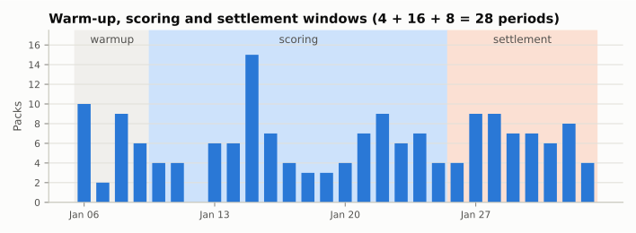
Window	Purpose	Orders allowed
Warm-up	Let the system move away from the opening state	yes
Scoring	The periods your metrics describe	yes
Settlement	Let late orders arrive and tails play out	only if `order_during_settlement=True`

Every window moves stock; only the scoring window counts by default. Each event table row carries its window in run_window.

Results¶

Setup: the tea shop from the Walkthrough

import numpy as np
import pandas as pd

from stockcast.core import InventoryStateDataFrame, SimulationEngine
from stockcast.policies import OrderUpToPolicy
from stockcast.utils import DemandGenerator

sku = "tea_250g"
opening_date = pd.Timestamp("2026-01-05")
lead_time, review_period = 2, 4
horizon = lead_time + review_period

demand = DemandGenerator(
    [sku], first_date=opening_date + pd.Timedelta(days=1), freq="D",
    random_seed=3, negative_demand_handling="clip_zero",
).seasonal(n_periods=56, base=6.0, amplitude=2.0, season_length=7, std=2.0)
demand["y"] = demand["y"].round()

inventory = InventoryStateDataFrame.from_observed(
    pd.DataFrame({"unique_id": [sku], "date": [opening_date], "on_hand": [30.0]}),
    allow_backorders=False,   # some pages step this state by hand
)

paths = np.random.default_rng(42).poisson(6.0, size=(10_000, horizon))


def tea_policy(probability):
    """Order-up-to policy whose target is the given quantile of 6-day demand."""
    target = pd.DataFrame({
        "unique_id": [sku],
        "target": [np.quantile(paths.sum(axis=1), probability)],
        "date": [opening_date + pd.Timedelta(days=horizon)],   # the last day it covers
    })
    return OrderUpToPolicy(
        lead_time=lead_time, review_period=review_period, freq="D",
        service_level=probability, allow_backorders=False,
    ).fit(target, target_column="target")


policy = tea_policy(0.95)
run_settings = dict(random_seed=3)
result = SimulationEngine().run(
    policy=policy, demand_source=demand, inventory=inventory, **run_settings,
)

Member	Returns
`to_event_frame(window=None)`	The event table, optionally one window (`"warmup"`, `"scoring"`, `"settlement"`, `"all"`)
`to_order_frame()`	One row per scheduled delivery: supplier, order and due periods, status
`to_callback_audit_frame()`	One row per accepted callback effect, with reason and source
`to_process_flow_frame()`	One row per inventory-process flow
`summary()`	A dict of headline numbers for the scoring window
`run_manifest`	The record of inputs, settings, and versions
`inventory`	The final state
`history`	State snapshots after each period

{key: round(float(value), 3) for key, value in result.summary().items()}

{'fill_rate': 1.0, 'demand_period_service_level': 1.0, 'mean_ending_on_hand_per_sku_period': 18.607, 'stockout_periods': 0.0, 'total_order_units': 333.0, 'order_event_count': 14.0, 'sku_order_line_count': 14.0}

The run manifest¶

Every result carries a manifest, a JSON-friendly dictionary with eight sections:

list(result.run_manifest)

['run_id', 'created_at_utc', 'demand_source', 'package', 'policy', 'opening_inventory', 'run_settings', 'dependencies']

Section	Records
`run_id`, `created_at_utc`	A unique id and timestamp
`demand_source`	Name, fingerprint, row count, seed, and generator settings of the demand
`package`, `dependencies`	Stockcast version (and source commit when available); Python, NumPy, pandas, and Matplotlib versions
`policy`	Policy class, configuration, target metadata, a fingerprint of the target table, and the fitted levels (`fitted_levels`: plain values when one value applies to every SKU, otherwise a fingerprint of the per-SKU table)
`opening_inventory`	A fingerprint of the opening state and open orders
`run_settings`	Frequency, windows, schedule, constraints, callbacks, supply, processes, timing convention, and `demand_period_offset`: the shift removed from a demand table's own period numbers (0 when none)

Store the manifest next to the event table and any result can be traced back to its inputs.

`run_comparison`¶

run_comparison runs several fitted policies on the same experiment. Name each one with a dict:

comparison = SimulationEngine().run_comparison(
    policies={"80%": tea_policy(0.80), "95%": tea_policy(0.95)},
    demand_source=demand,
    inventory=inventory,
    **run_settings,
)
comparison.summary()[["fill_rate", "mean_ending_on_hand_per_sku_period"]]

        fill_rate  mean_ending_on_hand_per_sku_period
policy
80%      0.994083                           13.964286
95%      1.000000                           18.607143

A list works too: policies=[a, b] with labels=["80%", "95%"], or without labels to use the policies' names.

The demand is built once and shared by every branch.
Each branch starts from its own copy of the opening state.
Constraints, callbacks, suppliers, and processes apply to every branch; callbacks and processes are reset between branches. Random supplier lead times use the same seeded draws per period and SKU. Seeded delivery outcomes follow each branch's own deliveries.
policy_schedules gives each branch its own refits: one per policy in list order, or {label: schedule} with a dict of policies.
allow_target_reuse and missing_targets apply to every branch.

comparison[label] is a normal SimulationResult; iterate over comparison for the labels.

Shelf life¶

FIFO shelf life is an inventory process: SimulationEngine().run(..., processes=[ShelfLife(shelf_life_days, opening_lots)]). See Shelf life and inventory processes.

Logging¶

SimulationEngine(verbose=1) prints start, end, and milestones; verbose=2 prints a line for every period.