Step 2 of 9

Demand and time¶

A simulation plays demand forward one period at a time. This page shows the demand table Stockcast reads and how periods map to calendar dates.

The demand table¶

Demand is a long table with one row per SKU and period:

Column	Meaning
`unique_id`	The SKU, matching the inventory state.
`period`	Zero-based period number: `0, 1, 2, …`
`date`	The calendar date of that period.
`y`	Units demanded in that period.

This is the same long format used by Nixtla's libraries and many other forecasting tools, so forecast outputs and demand tables line up naturally.

Periods and dates¶

The opening state has a date: the moment you counted the shelf. Demand period 0 is one step after it. With a daily frequency and an opening date of Monday 5 January, the calendar looks like this:

	Opening state	Period 0	Period 1	Period 2	…
Date	Mon 5 Jan	Tue 6 Jan	Wed 7 Jan	Thu 8 Jan	…

In general, period \(p\) is dated

\[ \text{date}_p = \text{opening date} + (p + 1)\,\Delta, \]

where \(\Delta\) is the period length, given as a pandas frequency: "D" for days, "W-MON" for weeks starting Monday, "h" for hours, and so on. Lead time and review period are counted in these periods.

Generate demand¶

DemandGenerator makes reproducible synthetic demand, which is handy for learning and for stress tests. The tea shop's eight weeks:

import pandas as pd

from stockcast.utils import DemandGenerator

sku = "tea_250g"
opening_date = pd.Timestamp("2026-01-05")

demand = DemandGenerator(
    [sku],
    first_date=opening_date + pd.Timedelta(days=1),   # date of period 0
    freq="D",
    random_seed=3,
    negative_demand_handling="clip_zero",
).seasonal(n_periods=56, base=6.0, amplitude=2.0, season_length=7, std=2.0)
demand["y"] = demand["y"].round()

demand.head()

  unique_id     y  period       date
0  tea_250g  10.0       0 2026-01-06
1  tea_250g   2.0       1 2026-01-07
2  tea_250g   9.0       2 2026-01-08
3  tea_250g   6.0       3 2026-01-09
4  tea_250g   4.0       4 2026-01-10

Eight weeks of tea demand

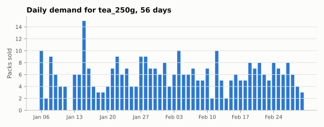
A normal distribution with a standard deviation of 2 can draw a negative value. negative_demand_handling="clip_zero" clips those draws to zero and tells you with a warning. The default, "raise", stops instead.

The generator also offers constant, normal, trend, normal_from_history (normal draws that match the mean and spread of your own history), and sample, which draws from any distribution you write as a small function.

Use your own data¶

Real sales history usually arrives wide or unlabelled. Reshape it into the long format; the dates are enough, and the engine numbers the periods for you:

sales = pd.DataFrame({
    "date": pd.date_range("2026-01-06", periods=4, freq="D"),
    "tea_250g": [10, 2, 9, 6],
    "coffee_1kg": [3, 4, 2, 5],
})

my_demand = sales.melt(id_vars="date", var_name="unique_id", value_name="y")
my_demand.head(4)

        date unique_id   y
0 2026-01-06  tea_250g  10
1 2026-01-07  tea_250g   2
2 2026-01-08  tea_250g   9
3 2026-01-09  tea_250g   6

Calendar checks¶

Before a run starts, the engine checks the whole calendar: every SKU appears in every period exactly once, the dates advance by exactly one frequency step, and every value is finite and non-negative. Days without sales are rows with y = 0.

Summary¶

Demand is a long table: unique_id, date (or a period number), y.
Period 0 is one frequency step after the opening state.
Lead times and review periods count periods, at the frequency you declare.

Next: Forecast targets