Order-up-to \((R, S)\)¶

The order-up-to policy is the standard rule for periodic replenishment. Every \(R\) periods it looks at the inventory position and orders enough to bring it back up to a target level \(S\).

The rule¶

At every decision period \(t\):

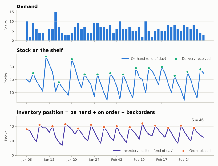
\[ q_t = \max\bigl(0,\; S_t - \mathit{IP}_t\bigr), \qquad \mathit{IP}_t = \mathit{OH}_t + P_t - B_t . \]

After the order, the inventory position equals \(S_t\) (unless it was already above). The picture shows the typical saw-tooth: the position climbs back to \(S\) at every review, and the shelf refills \(L\) periods later.

An order-up-to run

Choosing \(S\)¶

A decision at \(t\) must cover demand until the next order arrives, a window of \(H = L + R\) periods (derivation). With a target probability \(\alpha\):

\[ S = Q_\alpha\!\left(\sum_{h=0}^{H-1} D_{t+h}\right). \]

It is often useful to split \(S\) into expected demand and a buffer:

\[ S = \underbrace{\mathbb{E}\!\left[\textstyle\sum_h D_{t+h}\right]}_{\text{cycle and pipeline stock}} \;+\; \underbrace{\mathit{SS}}_{\text{safety stock}} . \]

For independent normal periods, \(\mathit{SS} = z_\alpha \sqrt{\sum_h \sigma_h^2}\), and for identical periods with standard deviation \(\sigma\) this is the textbook \(z_\alpha \sigma \sqrt{L + R}\) (Silver, Pyke and Thomas, 2017). Forecast targets covers every way of computing \(S\).

Orders replace demand¶

With backorders and an inventory position at or below \(S\) before each review, the order replaces what was sold since the last review:

\[ q_t = S - \mathit{IP}_t = S - (S - D_{t-R} - \dots - D_{t-1}) = \sum_{k=1}^{R} D_{t-k}. \]

Orders therefore pass demand variability straight through to the supplier, one reason the \((R, S)\) policy is easy to plan around.

In Stockcast¶

import numpy as np
import pandas as pd

from stockcast.policies import OrderUpToPolicy

opening_date = pd.Timestamp("2026-01-05")
target = pd.DataFrame({
    "unique_id": ["tea_250g"],
    "S": [46.0],
    "S_end": [opening_date + pd.Timedelta(days=6)],
})

policy = OrderUpToPolicy(
    lead_time=2,
    review_period=4,
    freq="D",
    service_level=0.95,
    allow_backorders=False,
    date_column="S_end",
).fit(
    target,
    target_column="S",
    forecast_origin=opening_date,
)
policy.get_target_metadata()

{'representation': 'direct_protection_period_target', 'target_probability': 0.95, 'protection_horizon': 6, 'target_source': 'external_direct', 'forecast_origin': '2026-01-05T00:00:00', 'forecast_frequency': 'D', 'target_end_date': '2026-01-11T00:00:00'}

Constructor¶

Argument	Meaning
`lead_time`	\(L\), integer \(\ge 0\)
`review_period`	\(R\), integer \(\ge 1\); or pass `schedule=` for other calendars
`freq`	\(\Delta\), the length of one period, such as `"D"`; optional when `fit` reads it from per-period forecast dates
`service_level`	\(\alpha\), or `None` for planner targets
`allow_backorders`	`True` or `False`
`schedule`	any `DecisionSchedule`
`sku_column`, `date_column`	column names of the tables given to `fit` and `predict` (defaults `"unique_id"`, `"date"`)

Fitting¶

fit accepts one of two modes, described in Forecast targets:

direct: target_column;
independent normal: mean_column and std_column, one row per step.

Both date their rows with the policy's date_column (default "date", set in the constructor next to sku_column): the last period each row covers. The origin follows from it, so forecast_origin is optional (and checked when you give both). The window protection_horizon defaults to \(L + R\) and the probability target_probability to the service_level; pass them only to have them checked.

Special cases¶

Setting	Behaviour
`review_period=1`	Order every period: a base-stock policy. \(H = L + 1\).
`lead_time=0`	Orders arrive immediately, before demand. \(H = R\).
`schedule=ExplicitSchedule(...)`	Irregular reviews; each decision needs a target for its own window (see Decision schedules).
`policy_schedule={...}` in `run`	Fresh targets at later decisions, e.g. rolling forecasts.

Notes¶

\((R, S)\) is simple, robust, and widely used. With lost sales it is a strong heuristic rather than the exact optimum; the optimal lost-sales policy is more complex (Janakiraman and Roundy, 2004).
Orders happen at every review in which demand occurred. If each order has a fixed cost, compare it with \((R, s, S)\), which skips small orders.

References¶

Silver, E. A., Pyke, D. F., and Thomas, D. J. (2017). Inventory and Production Management in Supply Chains (4th ed.). CRC Press.
Janakiraman, G., and Roundy, R. O. (2004). Lost-sales problems with stochastic lead times: convexity results for base-stock policies. Operations Research, 52(5), 795–803. doi:10.1287/opre.1040.0130