Reorder point \((s, Q)\) and \((s, S)\)¶

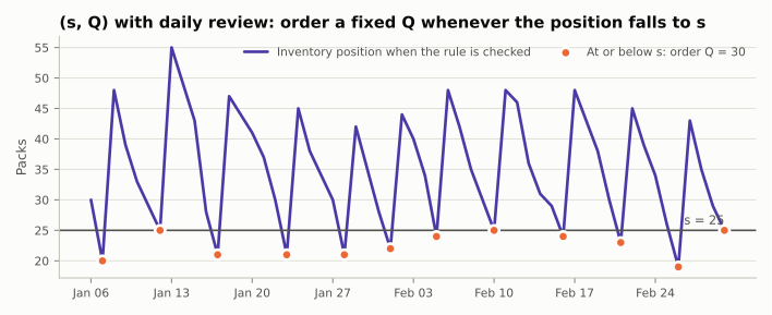
Reorder-point policies order only when stock gets low. At each opportunity they compare the inventory position with a reorder point \(s\). At or below it, they order. Above it, they wait.

The rules¶

At every decision period \(t\):

\[ (s, Q):\quad q_t = \begin{cases} Q & \text{if } \mathit{IP}_t \le s \\ 0 & \text{otherwise} \end{cases} \qquad\qquad (s, S):\quad q_t = \begin{cases} \max(0, S - \mathit{IP}_t) & \text{if } \mathit{IP}_t \le s \\ 0 & \text{otherwise} \end{cases} \]

\((s, Q)\) orders a fixed quantity: a pallet, a truckload, an economic order quantity.
\((s, S)\) orders up to a level \(S \ge s\), so larger drops get larger orders.

Reviewed every \(R\) periods, \((s, S)\) is the classic \((R, s, S)\) policy of periodic inventory control (Silver, Pyke and Thomas, 2017). With \(s = S\) it behaves like order-up-to \((R, S)\); lowering \(s\) skips small orders, which pays off when each order carries a fixed cost.

A reorder-point run

Choosing \(s\)¶

If the policy does not order at \(t\), the next chance is the next decision \(u\), and that order arrives at \(u + L\). The position at \(t\) must therefore cover demand over

\[ H = (u - t) + L \quad\Longrightarrow\quad H = L + R \ \text{(periodic)}, \qquad H = L + 1 \ \text{(every period)}, \]

and in quantile mode

\[ s = Q_\alpha\!\left(\sum_{h=0}^{H-1} D_{t+h}\right). \]

Note the \(L + 1\) for a policy reviewed every period, one more than the lead-time demand of continuous-review textbook formulas. Stockcast reviews once per period, before demand, so an order that is not placed today can only be placed tomorrow. Timing explains this in detail, and Notebook 05b shows how finer review steps approach the continuous-review result.

\(Q\) and \(S\) are ordering choices rather than quantiles. \(Q\) is often a pack size or an economic order quantity, and \(s\) and \(S\) are usually chosen together.

Where \(s\) and \(S\) come from¶

Reorder points come from many places: one house rule, a planning table, a forecast, a formula your team trusts. fit takes exactly one source:

You have	Pass to `fit`
one pair for every SKU	`reorder_point=20.0, order_up_to_level=50.0`
one value per SKU	`reorder_point={"tea_250g": 25.0, ...}` or a Series by SKU, such as `table["s"]`
a dated forecast quantile	a table with `reorder_point_column=...` (and `order_up_to_column=...`)
your own rule	a table with `target_provider=YourProvider()`

Every source goes through the same checks: finite values, \(s \ge 0\), and \(S \ge s\). Notebook 05g runs all of them on the same demand and compares them.

Fixed values¶

Pass the numbers directly. A dict or a Series gives one value per SKU:

import pandas as pd

from stockcast.core import InventoryStateDataFrame
from stockcast.policies import ReorderPointPolicy

opening_date = pd.Timestamp("2026-01-05")

policy = ReorderPointPolicy(
    lead_time=2, review_period=7, allow_backorders=False,
).fit(
    reorder_point={"tea_250g": 25.0, "coffee_1kg": 10.0},
    order_up_to_level={"tea_250g": 60.0, "coffee_1kg": 30.0},
)

state = InventoryStateDataFrame.from_observed(
    pd.DataFrame({"unique_id": ["tea_250g", "coffee_1kg"], "on_hand": [22.0, 14.0]}),
    opening_date=opening_date,
)
policy.predict(state, current_period=0).get_dataframe()[
    ["unique_id", "inventory_position", "reorder_point", "target_level", "order_quantity"]]

    unique_id  inventory_position  reorder_point  target_level  order_quantity
0    tea_250g                22.0           25.0          60.0            38.0
1  coffee_1kg                14.0           10.0          30.0             0.0

Tea is below its reorder point and orders up to 60; coffee is above its reorder point and waits.

The columns of a planning table work the same way, and a single number applies to every SKU:

table = pd.DataFrame({"unique_id": ["tea_250g", "coffee_1kg"],
                      "s": [25.0, 10.0], "S": [60.0, 30.0]}).set_index("unique_id")
from_table = ReorderPointPolicy(lead_time=2, review_period=7,
                                allow_backorders=False).fit(
    reorder_point=table["s"], order_up_to_level=table["S"],
)
house_rule = ReorderPointPolicy(lead_time=2, review_period=7,
                                allow_backorders=False).fit(
    reorder_point=20.0, order_up_to_level=50.0,
)

Fixed values are planning levels, so they need service_level=None (the default). Dates are optional: with forecast_origin (and the policy's freq), the run checks that the values were set no later than the first decision's information date. The run always needs the period length, so give the policy or the run a freq.

From a forecast¶

A forecast quantile is dated and covers a window, so the table carries the dates too. The window of \(s\) is checked at every decision.

(s, Q), quantile mode(s, S), planner mode

import numpy as np
import pandas as pd

from stockcast.policies import ReorderPointPolicy

opening_date = pd.Timestamp("2026-01-05")
L = 2
H = L + 1                       # review every period
totals = np.random.default_rng(42).poisson(6.0, size=(10_000, H)).sum(axis=1)

targets = pd.DataFrame({
    "unique_id": ["tea_250g"],
    "s": [np.quantile(totals, 0.95)],
    "s_end": [opening_date + pd.Timedelta(days=H)],
})

sQ = ReorderPointPolicy(
    lead_time=L,
    review_period=1,
    freq="D",
    policy_type="sQ",
    service_level=0.95,
    order_quantity=30.0,
    allow_backorders=False,
    date_column="s_end",
).fit(
    targets,
    forecast_origin=opening_date,
    reorder_point_column="s",
)
sQ.get_parameters()

  unique_id  reorder_point  order_quantity
0  tea_250g           25.0            30.0

When \(s\) and \(S\) come from an optimiser or a planning rule, set service_level=None:

planned = pd.DataFrame({
    "unique_id": ["tea_250g"],
    "s": [20.0],
    "S": [60.0],
    "s_end": [opening_date + pd.Timedelta(days=6)],
})
sS = ReorderPointPolicy(
    lead_time=2, review_period=4, freq="D", policy_type="sS",
    service_level=None, allow_backorders=False,
    date_column="s_end",
).fit(
    planned,
    forecast_origin=opening_date,
    reorder_point_column="s",
    order_up_to_column="S",
)
sS.get_parameters()

  unique_id  reorder_point  order_up_to_level
0  tea_250g           20.0               60.0

Your own rule¶

A target provider packages a rule of your own. It receives the table passed to fit and returns ReorderPointTargets(frame, metadata) with one row per SKU. Here \(s\) and \(S\) are days of cover of a daily rate:

from stockcast.policies import ReorderPointTargetProvider, ReorderPointTargets


class DaysOfCoverTargets(ReorderPointTargetProvider):
    """s = reorder_days x rate, S = order_up_to_days x rate."""

    def __init__(self, reorder_days, order_up_to_days):
        self.reorder_days, self.order_up_to_days = reorder_days, order_up_to_days

    def provide(self, target_data, *, sku_column):
        rate = target_data["daily_rate"]
        frame = pd.DataFrame({
            sku_column: target_data[sku_column],
            "reorder_point": self.reorder_days * rate,
            "order_up_to_level": self.order_up_to_days * rate,
        })
        return ReorderPointTargets(frame=frame, metadata=self.to_manifest())

    def to_manifest(self):
        return {**super().to_manifest(), "reorder_days": self.reorder_days,
                "order_up_to_days": self.order_up_to_days}


rates = pd.DataFrame({"unique_id": ["tea_250g", "coffee_1kg"], "daily_rate": [6.0, 2.0]})
cover = ReorderPointPolicy(lead_time=2, review_period=7, allow_backorders=False).fit(
    rates, target_provider=DaysOfCoverTargets(4, 10),
)
cover.get_parameters()

    unique_id  reorder_point  order_up_to_level
0    tea_250g           24.0               60.0
1  coffee_1kg            8.0               20.0

The provider's to_manifest() output is stored in the run manifest, so every result records how its levels were made. For an \((s, Q)\) policy, return reorder_point only. Set the class attribute target_source = "external_direct" when the provider only passes along values computed elsewhere; the default is "custom_provider". Like fixed values, provider levels need service_level=None and take optional dates.

Arguments¶

Constructor	Meaning
`policy_type`	`"sQ"` or `"sS"`; optional: giving `order_quantity` means `"sQ"`, otherwise `"sS"`
`lead_time`, `review_period` / `schedule`	as for every policy
`freq`	\(\Delta\), the length of one period; needed for column targets, optional for fixed values and providers
`service_level`	\(\alpha\) for quantile mode, `None` for planner mode
`order_quantity`	\(Q\); \((s, Q)\) only
`allow_backorders`	`True` or `False`
`sku_column`	SKU column of the tables given to `fit` and `predict` (default `"unique_id"`)
`date_column`	column with the last date covered by \(s\), origin \(+ H\Delta\) (default `"date"`); the origin follows from it. Column targets only

`fit`	Meaning
`reorder_point`	fixed \(s\): a number, a dict, or a Series by SKU
`order_up_to_level`	fixed \(S\), in the same forms; \((s, S)\) only
`target_provider`	a `ReorderPointTargetProvider`, called with the table
`reorder_point_column`	column holding \(s\)
`order_up_to_column`	column holding \(S\); \((s, S)\) only
`reorder_horizon`	\(H\): defaults to \(L + R\) for periodic schedules; required otherwise, checked as \((u - t) + L\)
`target_probability`	\(\alpha\), quantile mode only; defaults to `service_level`
`forecast_origin`	as for every target; optional for fixed values and providers

The window arguments (reorder_horizon, target_probability, order_up_to_column) and a named date_column belong to column targets.

Notes¶

Undershoot. Demand does not arrive one unit at a time. By the time the position is checked it may be well below \(s\). With \((s, Q)\) a single \(Q\) might then not lift it above \(s\) again; the policy orders \(Q\) once per opportunity. \((s, S)\) adapts the order size to the drop.
Reorder points and service. A quantile of window demand is the standard basis for \(s\). Realised service also depends on undershoot, \(Q\), and the shortage rule, which a simulation measures.