Step 8 of 9

Compare scenarios

Simulation is most useful for comparisons. Is a 95% target worth the extra stock over an 80% one? Is a better forecast worth more than a better ordering rule? A fair comparison runs every alternative on the same demand from the same starting point.

Setup: the tea shop from steps 1 to 5

import numpy as np
import pandas as pd

from stockcast.core import InventoryStateDataFrame, SimulationEngine
from stockcast.policies import OrderUpToPolicy
from stockcast.utils import DemandGenerator

sku = "tea_250g"
opening_date = pd.Timestamp("2026-01-05")
lead_time, review_period = 2, 4
horizon = lead_time + review_period

demand = DemandGenerator(
    [sku], first_date=opening_date + pd.Timedelta(days=1), freq="D",
    random_seed=3, negative_demand_handling="clip_zero",
).seasonal(n_periods=56, base=6.0, amplitude=2.0, season_length=7, std=2.0)
demand["y"] = demand["y"].round()

inventory = InventoryStateDataFrame.from_observed(
    pd.DataFrame({"unique_id": [sku], "date": [opening_date], "on_hand": [30.0]}),
    allow_backorders=False,   # some pages step this state by hand
)

paths = np.random.default_rng(42).poisson(6.0, size=(10_000, horizon))


def tea_policy(probability):
    """Order-up-to policy whose target is the given quantile of 6-day demand."""
    target = pd.DataFrame({
        "unique_id": [sku],
        "target": [np.quantile(paths.sum(axis=1), probability)],
        "date": [opening_date + pd.Timedelta(days=horizon)],   # the last day it covers
    })
    return OrderUpToPolicy(
        lead_time=lead_time, review_period=review_period, freq="D",
        service_level=probability, allow_backorders=False,
    ).fit(target, target_column="target")


policy = tea_policy(0.95)
run_settings = dict(random_seed=3)
result = SimulationEngine().run(
    policy=policy, demand_source=demand, inventory=inventory, **run_settings,
)

Compare three targets

run_comparison takes a list of fitted policies and runs each one on the same demand, each from its own fresh copy of the opening state:

from stockcast.core import SimulationEngine

comparison = SimulationEngine().run_comparison(
    policies=[tea_policy(0.50), tea_policy(0.80), tea_policy(0.95)],
    labels=["target 0.50", "target 0.80", "target 0.95"],
    demand_source=demand,
    inventory=inventory,
    **run_settings,
)
comparison.summary()[["fill_rate", "stockout_periods",
                      "mean_ending_on_hand_per_sku_period", "total_order_units"]]

             fill_rate  stockout_periods  mean_ending_on_hand_per_sku_period  total_order_units
policy
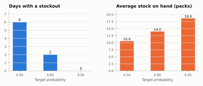
target 0.50   0.946746                 6                           10.571429              305.0
target 0.80   0.994083                 2                           13.964286              326.0
target 0.95   1.000000                 0                           18.607143              333.0

tea_policy(p) (in the setup above) sets the target to the \(p\)-quantile of six-day demand: 36, 41, and 46 packs. Higher targets buy service with stock:

Fair comparison

• One demand path. The demand is read once and shared by every branch.
• Separate stock. Each branch starts from its own copy of the opening state, so one policy's orders never leak into another's shelf.
• Same rules. Constraints, suppliers, callbacks, and processes you pass apply identically to every branch. Random supplier lead times are drawn once and shared, so branches differ only by the policy.

Differences in the results therefore come from the policies alone.

Costs

Service and stock pull in opposite directions. Costs put them on one scale. Each branch is a normal SimulationResult, so the evaluator works as in step 7:

import pandas as pd

from stockcast.evaluation import InventoryEvaluator, fill_rate, total_cost

costs = {
    "holding_cost_per_unit_period": 0.02,
    "shortage_cost_per_unit": 2.00,
    "order_cost_per_sku_line": 5.00,
    "order_cost_per_unit": 0.0,
    "cost_components": ["holding", "shortage", "ordering"],
}
scores = pd.concat({
    label: InventoryEvaluator().fit(comparison[label], window="scoring").evaluate(
        [fill_rate, total_cost], groupby=[], context=costs)
    for label in comparison
}).droplevel(1)
scores.round(3)

             fill_rate  total_cost
target 0.50      0.947      117.84
target 0.80      0.994       89.64
target 0.95      1.000       90.84

With lost margin at €2 per pack and shelf space at €0.02 a day, the 80% target is the cheapest of the three: its two small stockouts cost less than the extra stock the 95% target carries. The 50% target loses too many sales. Raise the lost margin and the 95% target wins.

Other comparisons

The same pattern compares anything that is a policy:

• two forecasting models, by fitting the same policy on each model's target;
• two ordering rules, such as order-up-to against a reorder point;
• a custom policy against a built-in one.

For longer studies with rolling forecasts, see Compare forecasts and policies and Notebook 06.

Summary

The research pipeline:

• run_comparison runs several policies on identical demand from identical, separate starting states.
• Differences in results come from the policies alone.
• Metrics and costs turn the comparison into a decision.

Next steps

• Step 9: From backtest to production runs the chosen policy as a daily job.
• The Guide covers each building block in depth.
• The Recipes answer specific questions.
• The Examples show larger workflows.

Next: From backtest to production