Step 5 of 9

The engine¶

SimulationEngine is the clock of a Stockcast run. It takes the demand, the opening state, and a fitted policy, and simulates them period by period. It is the only object that changes stock.

Order of events¶

Every period follows the same order: receive, decide, then meet demand.

flowchart LR
    A["1 · Receive<br/>deliveries due today<br/>arrive before opening"] --> B["2 · Decide<br/>on a review day, the policy<br/>sees the state and orders"]
    B --> C["3 · Meet demand<br/>serve customers;<br/>lost sales or backorders"]
    C --> D["Record<br/>one event table row per SKU,<br/>balances checked"]

Because the decision comes before demand, the policy never sees today's sales when it orders. An order placed in period \(t\) with lead time \(L\) is received at the start of period \(t + L\), in time for that period's demand. With \(L = 0\) it arrives immediately and can serve today's customers.

Timing of one decision

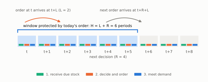
The coloured strips inside each day are the three moves. Today's order (at \(t\)) arrives at \(t + 2\). The next review is at \(t + 4\), and its order arrives at \(t + 6\). So today's order must cover demand on days \(t\) to \(t + 5\): the \(H = L + R\) window from step 3.

Run a simulation¶

import numpy as np
import pandas as pd

from stockcast.core import InventoryStateDataFrame, SimulationEngine
from stockcast.policies import OrderUpToPolicy
from stockcast.utils import DemandGenerator

sku = "tea_250g"
opening_date = pd.Timestamp("2026-01-05")
lead_time, review_period = 2, 4
horizon = lead_time + review_period

demand = DemandGenerator(
    [sku], first_date=opening_date + pd.Timedelta(days=1), freq="D",
    random_seed=3, negative_demand_handling="clip_zero",
).seasonal(n_periods=56, base=6.0, amplitude=2.0, season_length=7, std=2.0)
demand["y"] = demand["y"].round()

inventory = InventoryStateDataFrame.from_observed(
    pd.DataFrame({"unique_id": [sku], "date": [opening_date], "on_hand": [30.0]}),
)

paths = np.random.default_rng(42).poisson(6.0, size=(10_000, horizon))
target = pd.DataFrame({
    "unique_id": [sku],
    "target": [np.quantile(paths.sum(axis=1), 0.95)],
    "date": [opening_date + pd.Timedelta(days=horizon)],   # the last day it covers
})
policy = OrderUpToPolicy(
    lead_time=lead_time, review_period=review_period, freq="D",
    service_level=0.95, allow_backorders=False,
).fit(target, target_column="target")

engine = SimulationEngine()
result = engine.run(
    policy=policy,
    demand_source=demand,
    inventory=inventory,
    random_seed=3,
)
result

SimulationResult(policy=Order-Up-To (R,S), n_periods=56, history_rows=56)

The policy orders on periods 0, 4, 8, …: every \(R = 4\) periods, starting with the first. That rhythm is the policy's decision schedule. review_period=4 is shorthand for PeriodicSchedule(every=4); one-off and irregular calendars are covered in Decision schedules.

Inferred settings¶

run needs only the policy, the demand, and the opening state. It reads the rest from them and records it in the run manifest:

Setting	Read from	Set it yourself when
`n_periods`	the demand table's `period` column (here 56)	demand comes from a function
`freq`	the policy's `freq` (here `"D"`)	a custom policy has none
run windows	score every period	you want a warm-up or settlement window
`demand_source_name`, `random_seed`	not recorded	you want the manifest to name the demand or its seed

Run windows¶

A run can be split into three consecutive windows that add up to n_periods. Pass warmup_periods and settlement_periods; scoring gets the rest:

Run windows

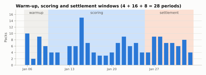
Warm-up lets the system settle, so the opening stock does not colour the results.
Scoring is the window your metrics describe.
Settlement plays demand a little longer, so orders placed near the end of scoring can arrive. With a settlement window, also say whether the policy may keep ordering there (order_during_settlement=True or False).

All three windows move stock. Only the scoring window counts by default.

Inputs are not modified¶

The engine copies the state and the policy before it starts. Your inventory and policy objects are unchanged after a run and can be reused:

inventory.inventory_position()[["on_hand", "inventory_position"]]

   on_hand  inventory_position
0     30.0                30.0

Run manifest¶

Each result carries a run manifest: the demand fingerprint, the policy and its target metadata, the opening state, every run setting, and the package versions. The manifest is stored with the result.

result.run_manifest["run_settings"]["decision_schedule"]

{'type': 'periodic', 'every': 4, 'start': 0}

Summary¶

Each period: receive → decide → meet demand, then record.
An order placed at \(t\) arrives at the start of \(t + L\).
run needs only the policy, the demand, and the opening state; it reads the run length and period length from them and never changes your input objects.

Next: The event table