Timing: receive, decide, demand
Inventory results depend on when things happen inside a period. Does a delivery arrive before or after today's customers? Does the policy see today's sales before it orders? This page defines the order of events that every part of Stockcast uses.
The sequence of events
Every period runs the same steps, in this order:
| Step | What happens | Who acts |
|---|---|---|
| 1. Open | Before-demand flows of inventory processes, such as expired lots leaving the shelf | InventoryProcess.before_demand (e.g. ShelfLife) |
| 2. Receive | Deliveries due this period arrive; old backorders are served first | engine (supplier DeliveryOutcomes decide what arrives) |
| 3. Decide | On a scheduled period, the policy proposes an order from the pre-demand state; callbacks, constraints, and the supply model shape it | DecisionSchedule, policy, on_after_prediction, OrderingConstraints, SupplyModel |
| 4. Place | \(L > 0\): the order enters the pipeline. \(L = 0\): it is received now | engine |
| 5. Meet demand | Serve customers from the shelf; the rest is lost or backordered | engine |
| 6. Close | After-demand process flows, then stock adjustments from callbacks | InventoryProcess.after_demand, on_after_demand |
| 7. Record | One event table row per SKU, with every balance identity checked | engine |
In one sentence: receive, decide, then meet demand. This is the classic periodic-review convention in the inventory literature: receive outstanding orders, review and order, then observe demand (see for example Zhu, 2022, Section 3).
What the policy sees
At step 3 the policy sees the state after today's deliveries and before
today's demand. Current-period flow fields are reset and the policy receives a
copy of the state, so today's demand is never visible when the decision is
made. The inventory position it sees is recorded in the event table as
decision_inventory_position.
When an order arrives
An order placed in period \(t\) is received at the start of period \(t + L\), before that period's demand.
| \(L\) | Placed in | Received | Can serve demand of |
|---|---|---|---|
| 0 | period \(t\) | period \(t\), immediately after the decision | period \(t\) |
| 1 | period \(t\) | start of period \(t + 1\) | period \(t + 1\) onwards |
| 2 | period \(t\) | start of period \(t + 2\) | period \(t + 2\) onwards |
Zero lead time is a legitimate and well-studied case: goods ordered in the morning are on the shelf before the shop opens (Dubois, Allaert and Witlox, 2013). A zero-lead-time order is recorded both as an order and as a receipt, and never enters the pipeline.
The protection horizon
Take a periodic policy that reviews every \(R\) periods with lead time \(L\), and a decision at period \(t\).
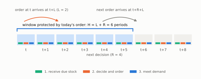
- The order placed now arrives at \(t + L\).
- The next decision is at \(t + R\). Its order arrives at \(t + R + L\).
- Nothing ordered later can arrive earlier than that.
So the inventory position right after today's order,
is all the stock that will be available for demand in periods \(t, t+1, \dots, t+R+L-1\). That window has
periods. This holds when new orders arrive exactly \(L\) periods after they are placed, all pipeline stock counted in \(\mathit{IP}_t^{+}\) arrives within the window, and nothing else moves stock in or out during it (no shelf-life write-offs, no stock changed by a callback). For opening orders, check their recorded arrival dates. With backorders, the net stock at the end of period \(t + H - 1\) is then \(\mathit{IP}_t^{+}\) minus the window's demand, so the window ends with no backlog exactly when that demand is at most \(\mathit{IP}_t^{+}\):
This is a statement about the end of the window. A shortage earlier in the window can still occur and be cleared when today's order arrives.
An order-up-to policy raises the position to \(\mathit{IP}_t^{+} = S\) whenever it starts at or below \(S\). Choosing \(S\) as the \(\alpha\)-quantile of total demand over the window,
makes that probability at least \(\alpha\), when the forecast distribution is the true one. It is exactly \(\alpha\) for continuous demand. For whole-unit demand the quantile is the smallest level whose probability reaches \(\alpha\), so the coverage can be above it. A position that is already above \(S\), or an order rounded up by a constraint, can increase that probability; an order capped by a constraint can decrease it. This is the familiar "lead time plus review period" protection interval of periodic review (Graves; Silver, Pyke and Thomas). The event sequence above fixes its exact endpoints. With lost sales the same target is the standard, widely used approximation. With unreliable deliveries or random lead times, orders no longer arrive on the policy's clock, so the probability above no longer holds as stated.
| \(L\) | \(R\) | \(H\) | Periods covered by a decision at \(t\) |
|---|---|---|---|
| 0 | 1 | 1 | \(t\) |
| 1 | 1 | 2 | \(t,\ t+1\) |
| 2 | 4 | 6 | \(t, \dots, t+5\) (the tea shop) |
| 7 | 7 | 14 | two weeks: one of lead time, one until the next order |
Coverage is about the position, not the shelf
The window starts at \(t\), before today's order arrives. Demand in periods \(t, \dots, t+L-1\) is served from stock already on the shelf or already on its way. A higher target today cannot help those first \(L\) periods. This is why the opening stock matters so much at the start of a run.
Irregular schedules
The same argument works for any deterministic schedule. If the next decision after \(t\) is at \(u\), the order placed at \(t\) must cover the periods until the order placed at \(u\) arrives:
With ExplicitSchedule([0, 3, 10]) and \(L = 2\), the decision at 0 covers
\(3 + 2 = 5\) periods and the decision at 3 covers \(7 + 2 = 9\). Different
decisions need targets for different windows; you supply one fitted policy per
decision with policy_schedule. When there is no next decision, you state the
final window explicitly. See Decision schedules.
Reorder points
A reorder-point policy asks, at each opportunity, "should I order now?" If it does not order at \(t\), the earliest help arrives from an order at \(u\), at \(u + L\). So its reorder point must cover the same window, \(H_t = (u - t) + L\). With review every period (\(u = t + 1\)):
That extra period, compared with continuous-review textbook formulas that use \(L\) alone, is the price of reviewing once per period before demand. Notebook 05b shows it numerically. See Reorder point.
Information: what a forecast may know
A decision in period \(t\) happens before period \(t\)'s demand. The latest demand it can know is that of period \(t - 1\). So the forecast origin for a decision in period \(t\) is
that is, the date of period \(t - 1\), or the opening date for \(t = 0\). The forecast's first step is period \(t\), and a target for horizon \(H\) ends at \(\text{origin}_t + H\Delta\). Stockcast checks these dates when you fit a policy, and again before the run starts for every scheduled decision, so each target lines up with the decision it is used for.
Two period counters
The event table carries two period columns, for two different jobs:
| Column | Counts | First value | Used by |
|---|---|---|---|
demand_period |
Rows of your demand table | 0 | Decision schedules, policy_schedule keys, the demand table's period |
period |
Steps of the inventory state | opening period + 1 | The state, callbacks (CallbackContext.period), current_period in predict |
With an opening state at period 0, period = demand_period + 1. Callbacks can
also match on date, which is often the simplest choice.
Other conventions you may meet
Papers and simulators differ in where they place the decision inside a
period, and in what their "lead time" counts. Each convention is valid, and
each maps exactly onto the clock on this page: an order placed at the end of
period \(t\) is Stockcast's order at the start of \(t + 1\).
Work with any timing convention walks
through the common cases, with the papers that use them. Stockcast's order
is the one on this page, everywhere, and the manifest of every run records
it as timing_convention.
How this is tested
The timing is pinned down by tests that compare the engine against an
independent, hand-written calendar of orders, arrivals, stock, and backorders
(tests/unit/test_decision_timing.py).
They cover lead times \(L = 0, 1, 2\) with review periods \(R = 1, 2, 3\) in both
shortage modes, irregular and one-time schedules, reorder-point windows,
zero-lead-time receipts with shelf life and backorders, constraints before
receipt, and the rule that a decision never sees current demand. A separate
reference model
(tests/unit/test_inventory_reference_model.py)
checks positive-lead-time runs and their evaluated costs. Outside the test
suite, the engine was compared with Stockpyl 1.0.2, which observes demand
before ordering: with Stockpyl's lead time one period longer, both place
identical orders in every period on the same demand, and Stockcast's
simulated costs for Stockpyl's exact optimal \((s, S)\) and \((r, Q)\) policies
agree with Stockpyl's cost formulas within simulation error.
References
- Zhu, H. (2022). A simple heuristic policy for stochastic inventory systems with both minimum and maximum order quantity requirements. Annals of Operations Research, 309, 347–363. doi:10.1007/s10479-021-04441-1
- Dubois, T., Allaert, G., and Witlox, F. (2013). Determining the fill rate for a periodic review inventory policy with capacitated replenishments, lost sales and zero lead time. Operations Research Letters, 41(6), 726–729. doi:10.1016/j.orl.2013.10.006
- Graves, S. C. Manufacturing system and supply chain design, MIT OpenCourseWare 15.763J (2005), summary slides.
- Silver, E. A., Pyke, D. F., and Thomas, D. J. (2017). Inventory and Production Management in Supply Chains (4th ed.). CRC Press.
- Stockpyl simulation: sequence of events
- SimOpt: (s, S) inventory model
See also: Work with any timing convention · Notebook 02b: decision schedules